First steps with SWAT+: what every beginner needs to know

Leia em português: Primeiros passos com o SWAT+

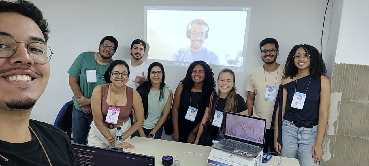
On 14 and 15 October 2026 (08:00-12:00 each day) I taught the short course “Introduction to SWAT+ for beginners” at the National Science and Technology Week (SNCT 2026) of IFBA, Vitória da Conquista campus, Brazil: 8 hours over two mornings, for students and professionals who had never used SWAT. This post brings together the main points covered in the course and tips for continued learning. It is a good starting point for beginners: it shows the path and the most common stumbling blocks in the first steps with SWAT+.

Participants of the MC07 short course at SNCT 2026, IFBA Vitória da Conquista. I taught the course remotely from Austria (on screen).

What SWAT+ is

SWAT+ (Soil and Water Assessment Tool Plus) is a watershed model that is continuous in time (daily time step), semi-distributed and process-based: most parameters come from soil, land use and topography and have physical meaning, although some components are empirical (for example, the Curve Number method for surface runoff). It estimates streamflow, the water balance, sediments, nutrients and the effect of management, land-use and climate scenarios.

SWAT+ is a complete restructuring of SWAT 2012, developed by USDA-ARS and Texas A&M University (Bieger et al., 2017). Most process equations come from SWAT 2012 (Neitsch et al., 2011); the organisation is different:

Aspect	SWAT 2012	SWAT+
GIS interface	ArcSWAT (ArcGIS, commercial) or QSWAT	QSWAT+ (QGIS, free)
Database	Microsoft Access	SQLite
Connections between units	fig.fig file, rigid	Connect files (.con), flexible
Spatial hierarchy	Watershed, subbasins, HRUs	Watershed, subbasins, landscape units (LSUs), HRUs and water areas
Management	By date or heat units	Also by decision tables
Calibration	Edits the input files	calibration.cal overrides values without changing the originals

The unit of calculation is still the HRU (hydrologic response unit): a unique combination of landscape unit, land use, soil and slope class. An HRU has no continuous location; it is the sum of all cells with the same combination.

Three programs, one model

The first source of confusion is that SWAT+ is in practice a set of three programs:

Component	What it does
QSWAT+ (QGIS plugin)	Builds the spatial part: delineates the watershed, creates LSUs and HRUs, visualises results. It is not the model.
SWAT+ Editor	Imports climate data, sets the period, options and outputs, writes the text files and runs the model
SWAT+ (executable)	The model itself: reads the text files in TxtInOut and writes the outputs

Everything comes with the official SWAT+ installer. The model source code is archived on Zenodo (Arnold et al., 2026). Use the 64-bit QGIS LTR, the version tested by the developers, and tick the optional global weather generator download during installation.

The data you need

A basic model needs five datasets, all in the same metric projection:

Data	Purpose	Example sources (Brazil)
Digital elevation model	Drainage, subbasins, slope	ANADEM, Copernicus GLO-30, SRTM 30 m, TOPODATA (INPE)
Land use and land cover	Plants, Curve Number and management for each HRU	MapBiomas (annual collections, 30 m)
Soils	Layers, texture, available water, conductivity	IBGE and Embrapa maps; SoilGrids to fill in properties
Daily climate	Precipitation, temperature, radiation, humidity, wind	INMET (BDMEP), ANA Hidroweb, BR-DWGD grid, CHIRPS, ERA5
Observed streamflow	Evaluation, calibration and validation	ANA Hidroweb / SNIRH

For delineation, prefer a terrain model such as ANADEM (Laipelt et al., 2024), which reduces the vegetation bias of Copernicus GLO-30: surface models such as SRTM and Copernicus partly include canopy height, which can shift the drainage network in forested areas.

In practice, the hardest dataset is almost always the soil property table (usersoil): depth, bulk density, available water and conductivity for every layer.

Two rules prevent most errors:

• QSWAT+ assumes all cells have the same area. A DEM in degrees (latitude/longitude) must be reprojected first, to the UTM zone of the watershed (in Brazil, SIRGAS 2000 / UTM) or to an equal-area projection for basins that cross UTM zones.
• Folder and file names without spaces, accents or special characters.

Lessons from a real project with Brazilian data:

• Hidroweb streamflow: use only the checked (consistido, consistency level 2) series and read the status code of each day (1 real, 2 estimated, 3 doubtful, 4 dry gauge). At some stations, whole years are estimated; evaluate the model on real-status days. CAMELS-BR is a useful cross-check.
• Station metadata is not always right: reported drainage areas can be wrong and old coordinates may be rounded. Check the area against your delineation.
• BR-DWGD gridded rainfall (Xavier et al., 2022): in that project it matched gauges in totals and timing, but had too many light-rain days and too few heavy ones. With the Curve Number method that means less surface runoff, which calibration then hides. Compare wet-day and heavy-rain frequencies with ANA gauges before using it.
• ZARC sowing windows are insurance periods, not observed practice: use Conab crop progress for real sowing dates and IBGE PAM yields to check crop growth.

Checklist before opening QSWAT+

Half an hour of checking here saves hours later:

• DEM, land use and soil maps share the same projected coordinate system
• The DEM’s vertical unit is metres
• Land use and soil cover the whole watershed, with no NoData holes
• Every land-use raster value has a row in the land-use lookup table; an unknown class stops the work instead of defaulting to pasture
• Every soil raster value exists in the soil lookup table, and every soil exists in usersoil
• The outlet lies on (or within 300 m of) the generated drainage network
• The climate record covers the simulation period plus the warm-up years
• Station coordinates are in decimal degrees, negative for South and West
• A reused example project does not carry a leftover calibration.cal

The workflow in six steps

1. Create the project in QSWAT+ (SWAT+ button in QGIS, New Project).
2. Delineate the watershed: load the DEM, set the channel and stream thresholds (smaller thresholds give more subbasins and a slower model), and add the outlet. Set the thresholds yourself (the defaults depend on the DEM size), then check every outlet: count how many snapped, and compare the delineated drainage area with the gauge’s (as a rule of thumb, a ratio outside 0.8-1.25 means the point is in the wrong place).
3. Create landscape units: separate floodplain and upslope areas (the DEM inversion method with default values is a good start).
4. Generate HRUs: land-use and soil maps with their lookup tables, slope classes, and a filter to drop small combinations (for example 10% for land use, soil and slope). Compare each land use’s area before and after filtering: the filter can quietly absorb minority covers such as pasture or plantations. Protect them with Exempt landuses.
5. Configure in the SWAT+ Editor: import the weather generator and observed climate, set the period and the warm-up years (1 to 3), and choose the outputs.
6. Run and check: a successful run ends with Execution successfully completed in simulation.out. Then use SWAT+ Check, which flags suspicious values (but does not tell you the model is wrong).

To learn, start with the Robit example dataset (Ethiopia) that comes with the installer: it lets you separate software problems from problems in your own data.

Common errors and where to look

Symptom	Likely cause
The outlet does not snap to the drainage (0 snapped)	Point too far from the network, or stream threshold too large
Error reading land use or soil	Raster value missing from the lookup table, or different projections
No rain anywhere	Station coordinates outside the watershed (sign of latitude/longitude)
Almost all flow is surface runoff	Curve Numbers too high, or wrong hydrologic soil group
Crops do not grow	No management assigned, or planting outside the period
The model stops right away	Climate does not cover the period, or a referenced file is missing
The run “succeeds” but results look odd	SWAT+ silently skips unknown names and missing weather files: search diagnostics.out for “not found”
Baseflow disappears in dry spells	Water-table depth threshold (flo_min, in aquifer.aqu) too shallow: groundwater only flows when the water table is within flo_min of the surface

Before calibrating: does the water balance make sense?

A model with a beautiful hydrograph and an absurd water balance is right for the wrong reasons. Before comparing with observed streamflow, open basin_wb_aa.txt (average annual watershed balance) and check:

• Closure (soil water balance): precipitation ≈ evapotranspiration + surface runoff + lateral flow + percolation + change in storage.
• ET/P consistent with the regional climate (ET higher than precipitation is a red flag, unless irrigation or groundwater supplies the difference).
• Flow partitioning: in a perennial watershed with an aquifer, nearly all flow as surface runoff points to Curve Numbers that are too high.
• Vegetation: near-zero biomass in agricultural HRUs points to a management problem.
• Plausibility: forest ET should usually exceed cropland ET, and simulated yields should be near the municipal PAM yields.
• Floodplain and upslope units: with these landscape units, upslope runoff that runs on to the floodplain can be counted twice in surq_gen of basin_wb; close the balance with HRU, aquifer and channel outputs instead, and check this in your SWAT+ version.

Only then comes calibration: first soft calibration (matching the water-balance fractions to regional values), then hard calibration against observed streamflow, and finally validation on an independent period. As a reference for monthly streamflow, Moriasi et al. (2007) consider NSE > 0.50, |PBIAS| < 25% and RSR ≤ 0.70 satisfactory. Treat these thresholds as a convention for comparing runs, not as proof that a model is fit for purpose. NSE and KGE (Gupta et al., 2009) are dominated by high flows, so also check hydrological signatures: the flow duration curve, Q95, the baseflow index and the monthly regime. Calibrate crop growth and evapotranspiration before streamflow, too: crop calibration changes the simulated water, sediment and nutrient results (Piniewski et al., 2026).

Keep learning

• The official SWAT+ page and the documentation, with a reference for every input and output file.
• The QSWAT+ tutorial and the SWAT+ Editor manual, installed with the software.
• The SWAT+ user group and the annual SWAT conferences.
• After your first model: decision tables for management, automatic calibration, and land-use and climate scenarios.
• A complete SWAT+ workflow, step by step: the OPTAIN CS10 documentation by Moritz Shore and colleagues documents a reproducible SWAT+ setup for the Kråkstad catchment (Norway), from input data and model setup to management, model verification, soft and hard calibration, and land-use, climate and measure scenarios. It is a work in progress, but an excellent guide to the steps that come after your first model.
• The OPTAIN project: project website and Zenodo community, with protocols, reports and data. Highlights: the SWAT+ modelling protocol applied in 14 European agricultural catchments (Schürz et al., 2022), the common optimisation protocol for water and nutrient retention measures (Strauch & Schürz, 2024) and the field-scale SWAP modelling protocol (Farkas et al., 2023): good examples of how to document a modelling study.
• R packages from the OPTAIN workflow: SWATprepR (input data preparation), SWATfarmR (management schedules) and SWATrunR (running and calibrating SWAT+ from R; formerly SWATplusR). There is also an R workflow to generate SWATfarmR input from field-scale crop rotations (Strauch, 2025). SWATbuildR and SWATdoctR are part of the workflow too, with restricted access.
• Calibrating crops, not just streamflow: Piniewski et al. (2026) show a crop growth and yield calibration workflow for SWAT+ and its effect on water, sediment and nutrient results in ten catchments.

References

• Arnold, J. G., Čerkasova, N., White, M., et al. (2026). Soil and Water Assessment Tool Plus (SWAT+) [Software]. Zenodo. doi:10.5281/zenodo.14983533
• Bieger, K., Arnold, J. G., Rathjens, H., White, M. J., Bosch, D. D., Allen, P. M., Volk, M., & Srinivasan, R. (2017). Introduction to SWAT+, a completely restructured version of the Soil and Water Assessment Tool. Journal of the American Water Resources Association, 53(1), 115-130. doi:10.1111/1752-1688.12482
• Chagas, V. B. M., et al. (2020). CAMELS-BR: hydrometeorological time series and landscape attributes for 897 catchments in Brazil. Earth System Science Data, 12(3), 2075-2096. doi:10.5194/essd-12-2075-2020
• Farkas, C., Shore, M., Cüceloglu, G., Czelnai, L., Nemes, A., Szabó, B., Čerkasova, N., Idzelyté, R., & Weiland, S. (2023). SWAP field-scale modelling protocol. OPTAIN project deliverable. Zenodo. doi:10.5281/zenodo.7907114
• Gupta, H. V., Kling, H., Yilmaz, K. K., & Martinez, G. F. (2009). Decomposition of the mean squared error and NSE performance criteria: implications for improving hydrological modelling. Journal of Hydrology, 377(1-2), 80-91. doi:10.1016/j.jhydrol.2009.08.003
• Laipelt, L., Comini de Andrade, B., Collischonn, W., de Amorim Teixeira, A., Paiva, R. C. D., & Ruhoff, A. (2024). ANADEM: A digital terrain model for South America. Remote Sensing, 16(13), 2321. doi:10.3390/rs16132321
• Moriasi, D. N., Arnold, J. G., Van Liew, M. W., Bingner, R. L., Harmel, R. D., & Veith, T. L. (2007). Model evaluation guidelines for systematic quantification of accuracy in watershed simulations. Transactions of the ASABE, 50(3), 885-900. doi:10.13031/2013.23153
• Neitsch, S. L., Arnold, J. G., Kiniry, J. R., & Williams, J. R. (2011). Soil and Water Assessment Tool Theoretical Documentation, Version 2009. Texas A&M University.
• Piniewski, M., Čerkasova, N., Plunge, S., Strauch, M., Schürz, C., et al. (2026). Enhanced crop calibration for SWAT+: evaluating water, sediment and nutrient impacts across ten European catchments. Environmental Modelling & Software, 196, 106794. doi:10.1016/j.envsoft.2025.106794
• Schürz, C., Čerkasova, N., Farkas, C., Nemes, A., Plunge, S., Strauch, M., Szabó, B., & Piniewski, M. (2022). SWAT+ modeling protocol for the assessment of water and nutrient retention measures in small agricultural catchments. OPTAIN project deliverable. Zenodo. doi:10.5281/zenodo.7463395
• Strauch, M. (2025). R workflow to generate SWATfarmR input (v1.0) [Software]. Zenodo. doi:10.5281/zenodo.17531016
• Strauch, M., & Schürz, C. (2024). Common optimisation protocol. Deliverable D5.1 of the EU Horizon 2020 project OPTAIN. Zenodo. doi:10.5281/zenodo.11473793
• Xavier, A. C., Scanlon, B. R., King, C. W., & Alves, A. I. (2022). New improved Brazilian daily weather gridded data (1961-2020). International Journal of Climatology, 42(16), 8390-8404. doi:10.1002/joc.7731